09. The Simplest Neural Network

Hi, it's Mat again!
The simplest neural network
So far you've been working with perceptrons where the output is always one or zero. The input to the output unit is passed through an activation function, f(h), in this case, the step function.
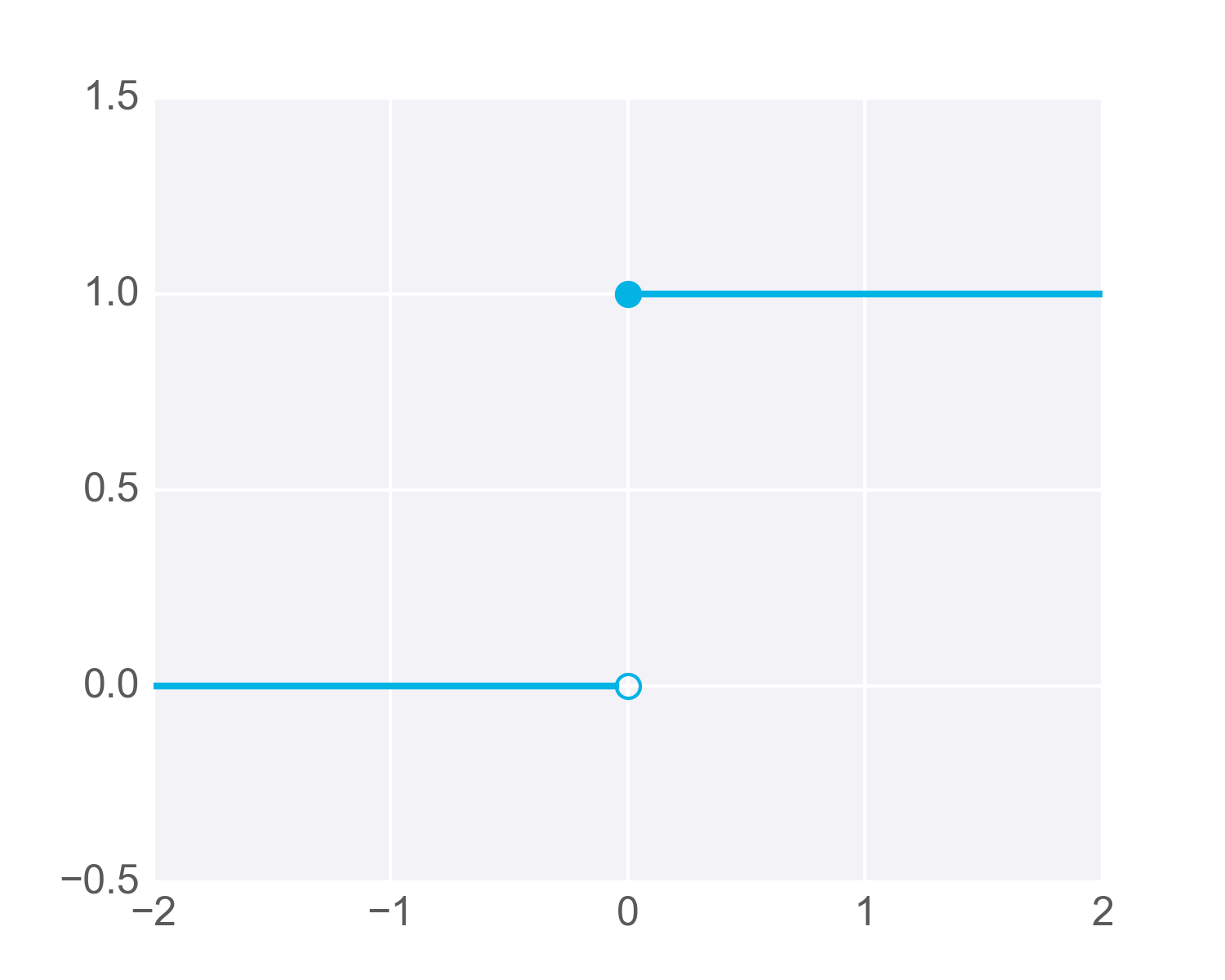
The step activation function.
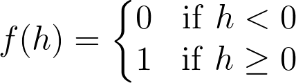
The output unit returns the result of f(h), where h is the input to the output unit:
h = \sum_i w_ix_i + b
The diagram below shows a simple network. The linear combination of the weights, inputs, and bias form the input h, which passes through the activation function f(h), giving the final output of the perceptron, labeled y.
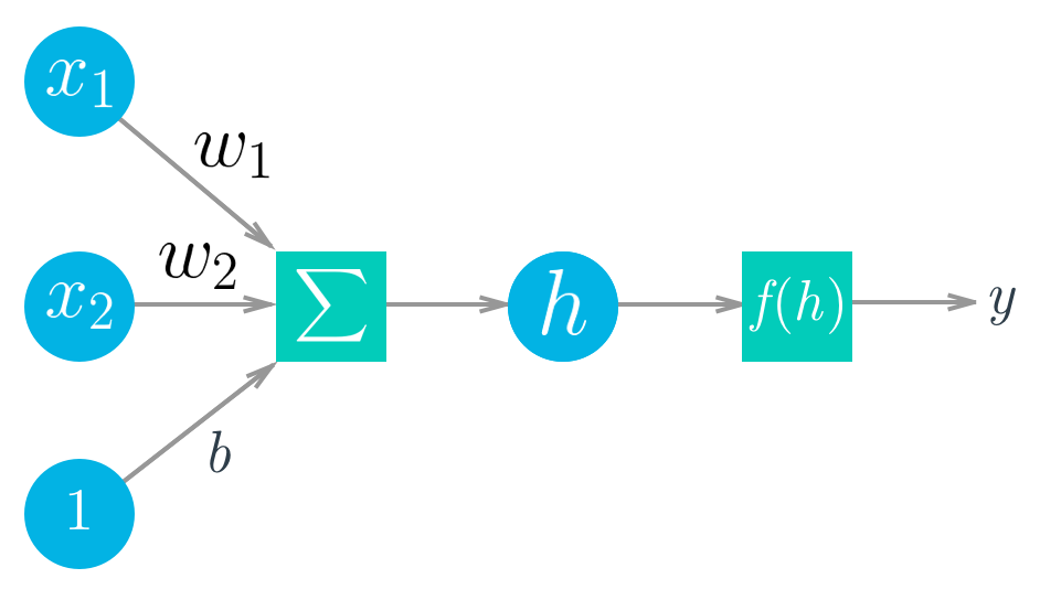
Diagram of a simple neural network. Circles are units, boxes are operations.
The cool part about this architecture, and what makes neural networks possible, is that the activation function, f(h) can be any function, not just the step function shown earlier.
For example, if you let f(h) = h, the output will be the same as the input. Now the output of the network is
y = \sum_iw_ix_i + b
This equation should be familiar to you, it's the same as the linear regression model!
Other activation functions you'll see are the logistic (often called the sigmoid), tanh, and softmax functions. We'll mostly be using the sigmoid function for the rest of this lesson:
\mathrm{sigmoid}(x) = 1/(1+e^{-x})
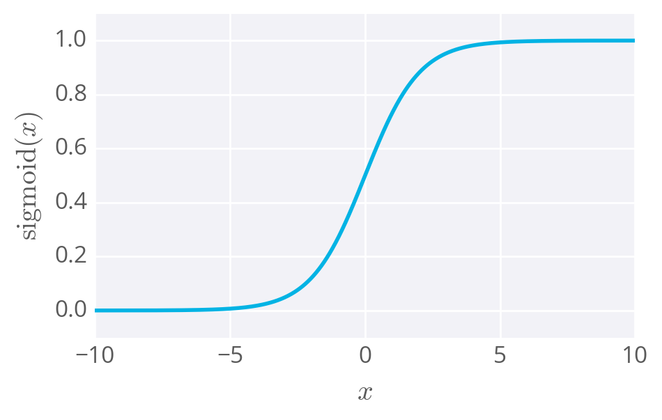
The sigmoid function
The sigmoid function is bounded between 0 and 1, and as an output can be interpreted as a probability for success. It turns out, again, using a sigmoid as the activation function results in the same formulation as logistic regression.
This is where it stops being a perceptron and begins being called a neural network. In the case of simple networks like this, neural networks don't offer any advantage over general linear models such as logistic regression.
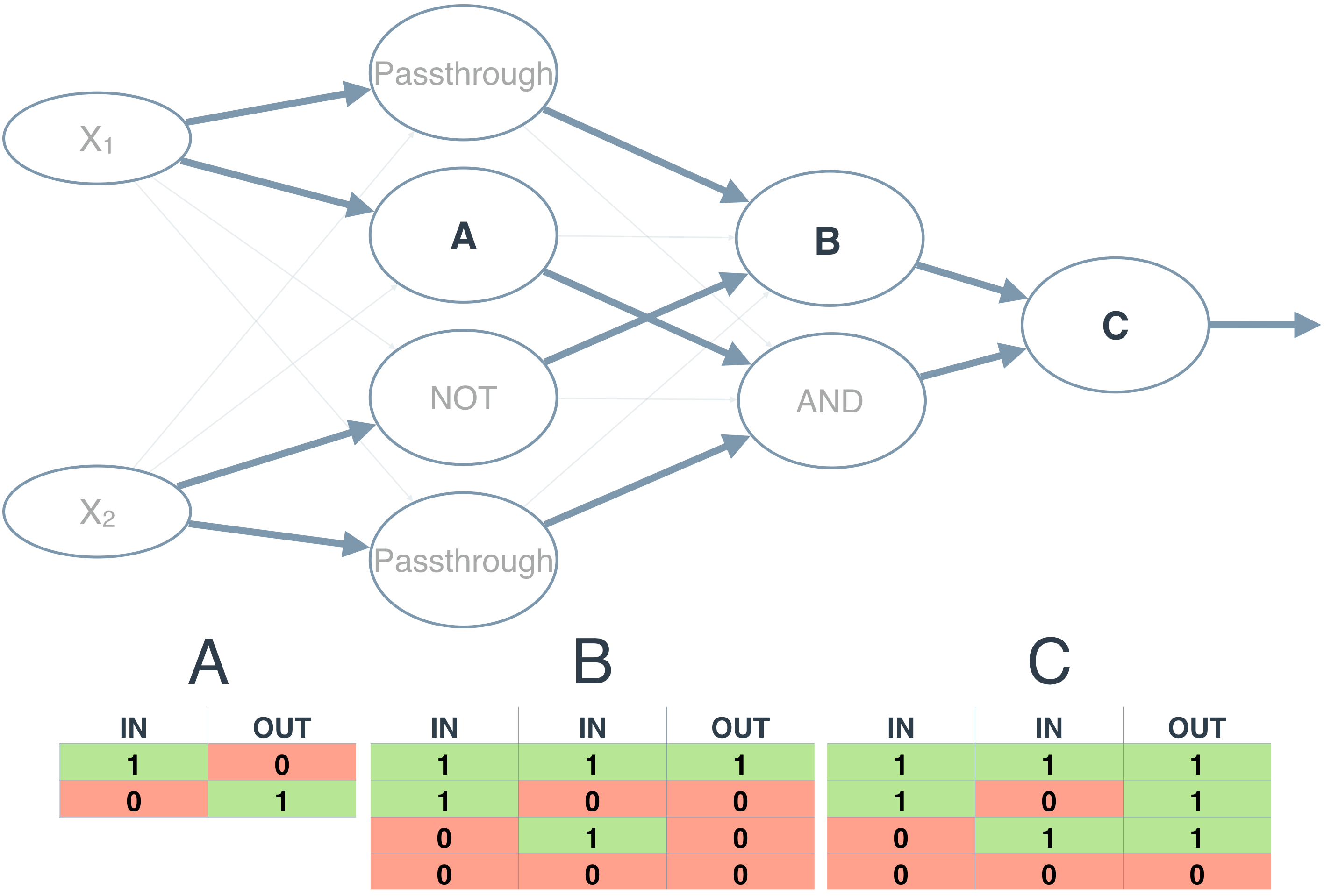
As you saw earlier in the XOR perceptron, stacking units lets us model linearly inseparable data.
But, as you saw with the XOR perceptron, stacking units will let you model linearly inseparable data, impossible to do with regression models.
Once you start using activation functions that are continuous and differentiable, it's possible to train the network using gradient descent, which you'll learn about next.
Simple network exercise
Below you'll use Numpy to calculate the output of a simple network with two input nodes and one output node with a sigmoid activation function. Things you'll need to do:
- Implement the sigmoid function.
- Calculate the output of the network.
As a reminder, the sigmoid function is
\mathrm{sigmoid}(x) = 1/(1+e^{-x})
For the exponential, you can use Numpy's exponential function, np.exp.
And the output of the network is
y = f(h) = \mathrm{sigmoid}(\sum_i w_i x_i + b)
For the weights sum, you can do a simple element-wise multiplication and sum, or use Numpy's dot product function.
Start Quiz: